Data Preparation for Machine Learning

<p>Data preparation consists in data collection, wrangling, and finally enfranchisement, if required and when possible.</p> <h2>Data collection</h2> <p>First, gather the data you will need for Machine Learning. Make sure you collect them in consolidated form, so that they are all contained within a single table (Flat Table).</p> <p>You can do this with whatever tool you are comfortable using, for example:</p> <ul> <li>Relational database tools (SQL)</li> <li>Jupiter notebook</li> <li>Excel</li> <li>Azure ML</li> <li>R Studio</li> </ul> <h2>Data wrangling</h2> <p>This involves preparing the data to make them usable by Machine Learning algorithms. <em>(Data Cleansing, Data Decomposition, Data Aggregation, Data Shaping and Transformation, Data Scaling.)</em></p> <h3><em>Data Cleansing</em></h3> <p>Find all the “Null” values, missing values and duplicate data.</p> <p>Examples of missing values:</p> <ul> <li>blanks</li> <li>NULL</li> <li>?</li> <li>N/A, NaN, NA</li> <li>9999999</li> <li>Unknown</li> </ul> <p> </p> <div> <table cellspacing="0" cellpadding="0"> <tbody> <tr> <th>#Row</th> <th>Title</th> <th>Type</th> <th>Format</th> <th>Price</th> <th>Pages</th> <th>NumberSales</th> </tr> <tr> <td>1</td> <td>Kids learning book</td> <td>Series – Learning – Kids -</td> <td>Big</td> <td>16</td> <td>100</td> <td>10</td> </tr> <tr> <td>2</td> <td>Guts</td> <td>One Book – Story - Kids</td> <td>Big</td> <td> </td> <td> </td> <td>3</td> </tr> <tr> <td>3</td> <td>Writing book</td> <td>Adults – learning- Series</td> <td> </td> <td>10</td> <td>120</td> <td>8</td> </tr> <tr> <td>5</td> <td>Dictation</td> <td>Series - Teenagers</td> <td>Small</td> <td>13</td> <td>85</td> <td>22</td> </tr> </tbody> </table> </div> <p><code>data_frame</code> below is our Pandas dataset:</p> <pre><code>#Count the number of missing values in each row in Pandas dataframedata_frame.isnull().sum()</code></pre> <pre><code>#Row 0Title 0Type 0Price 1Format 1Pages 1NumberSales 0</code></pre> <p>If certain rows are missing data in many important columns, we may consider removing these rows, using <code>DELETE</code> query in SQL or <code>pandas.drop()</code> in Python.</p> <p>Sometimes, the missing value can be replaced by either zero, the main common value, or the average value, depending on the column values and type. You can do this by using <code>UPDATE</code> query in SQL or <code>pandas.fillna()</code> in Python.</p> <p>In the following code, we have replaced the missing values of “Pages” with the mean:</p> <pre><code>global_mean = data_frame.mean()data_frame['Pages'] = data_frame['Pages'].fillna(global_mean['Pages'])data_frame.isnull().sum()</code></pre> <pre><code>#Row 0Title 0Type 0Price 1Format 1Pages 0NumberSales 0</code></pre> <p>And the missing “Format” values with the common value:</p> <pre><code>#Counts of unique valuesdata_frame["Format"].value_counts()</code></pre> <pre><code>Big 2Small 1Name: Format, dtype: int64</code></pre> <p>As “Big” is the most common value in this case, we have replaced all the missing values by “Big”.</p> <pre><code># Replace missing "Format" value with the most common value “Big”data_frame["Format"] = data_frame['Format'].fillna("Big")data_frame["Format"].value_counts()</code></pre> <pre><code>Big 3Small 1</code></pre> <p>The resulting data_frame is as follows:</p> <div> <table cellspacing="0" cellpadding="0"> <tbody> <tr> <th>#Row</th> <th>Title</th> <th>Type</th> <th>Format</th> <th>Price</th> <th>Pages</th> <th>NumberSales</th> </tr> <tr> <td>1</td> <td>Kids learning book</td> <td>Series – Learning – Kids -</td> <td>Big</td> <td>16</td> <td>100</td> <td>10</td> </tr> <tr> <td>2</td> <td>Guts</td> <td>One Book – Story - Kids</td> <td>Big</td> <td>13</td> <td>100</td> <td>3</td> </tr> <tr> <td>3</td> <td>Writing book</td> <td>Adults – learning- Series</td> <td>Big</td> <td>10</td> <td>120</td> <td>8</td> </tr> <tr> <td>4</td> <td>Dictation</td> <td>Series - Teenagers</td> <td>Small</td> <td>13</td> <td>85</td> <td>22</td> </tr> </tbody> </table> </div> <p>Make sure you have no duplicates. Delete duplicated rows using <code>DELETE</code> in SQL or <code>pandas.drop()</code> in Python.</p> <h3><em>Data Decomposition</em></h3> <p>If some of your text columns contain several items of information, split them up in as many dedicated columns as necessary. If some columns represent categories, convert them into dedicated category columns.</p> <p>In our example, the “Type” column contains more than one item of information, which can clearly be split into 3 columns, as shown below (Style, Kind and Readers). Then go through the same process as above for any missing values.</p> <div> <table cellspacing="0" cellpadding="0"> <tbody> <tr> <th>#Row</th> <th>Title</th> <th>Style</th> <th>Kind</th> <th>Readers</th> <th>Format</th> <th>Price</th> <th>Pages</th> <th>SalesMonth</th> <th>SalesYear</th> <th>NumberSales</th> </tr> <tr> <td>1</td> <td>Kids learning book</td> <td>Series</td> <td>Learning</td> <td>Kids</td> <td>Big</td> <td>16</td> <td>100</td> <td>11</td> <td>2019</td> <td>10</td> </tr> <tr> <td>2</td> <td>Guts</td> <td>One Book</td> <td>Story</td> <td>Kids</td> <td>Big</td> <td>13</td> <td>100</td> <td>12</td> <td>2019</td> <td>3</td> </tr> <tr> <td>3</td> <td>Writing book</td> <td>Series</td> <td>learning</td> <td>Adults</td> <td>Big</td> <td>10</td> <td>120</td> <td>10</td> <td>2019</td> <td>8</td> </tr> <tr> <td>4</td> <td>Writing book</td> <td>Series</td> <td>learning</td> <td>Adults</td> <td>Big</td> <td>10</td> <td>120</td> <td>11</td> <td>2019</td> <td>13</td> </tr> <tr> <td>5</td> <td>Dictation</td> <td>Series</td> <td>learning</td> <td>Teenagers</td> <td>Small</td> <td>13</td> <td>85</td> <td>9</td> <td>2019</td> <td>17</td> </tr> <tr> <td>6</td> <td>Dictation</td> <td>Series</td> <td>learning</td> <td>Teenagers</td> <td>Small</td> <td>13</td> <td>85</td> <td>10</td> <td>2019</td> <td>22</td> </tr> </tbody> </table> </div> <h3><em>Data Aggregation</em></h3> <p>This involves grouping data together, as appropriate.</p> <p>In our example, “Number of sales” is actually an aggregation of data. Initially, the database showed transactional rows, which we aggregated to obtain the number of books sold per month.</p> <h3><em>Data Shaping and Transformation</em></h3> <p>This involves converting categorical data to numerical data, since algorithms can only use numerical values.</p> <p>“Style”, “Kind”, “Readers” and “Format” are clearly categorical data. Below are two ways to transform them into numerical data.</p> <p><strong>1. 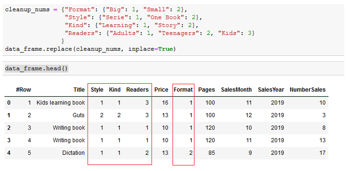<em>Convert all the categorical values to numerical values:</em></strong> Replace all unique values by sequential numbers.</p> <p>Example of how to do this in Python:</p> <pre><code>cleanup_nums = {"Format": {"Big": 1, "Small": 2}, "Style": {"Serie": 1, "One Book": 2}, "Kind": {"Learning": 1, "Story": 2}, "Readers": {"Adults": 1, "Teenagers": 2, "Kids": 3} }data_frame.replace(cleanup_nums, inplace=True)data_frame.head()</code></pre> <p>Result:</p> <div> <table cellspacing="0" cellpadding="0"> <tbody> <tr> <th>#Row</th> <th>Title</th> <th>Style</th> <th>Kind</th> <th>Readers</th> <th>Format</th> <th>Price</th> <th>Pages</th> <th>SalesMonth</th> <th>SalesYear</th> <th>NumberSales</th> </tr> <tr> <td>1</td> <td>Kids learning book</td> <td>1</td> <td>1</td> <td>3</td> <td>1</td> <td>16 $</td> <td>100</td> <td>11</td> <td>2019</td> <td>10</td> </tr> <tr> <td>2</td> <td>Guts</td> <td>2</td> <td>2</td> <td>3</td> <td>1</td> <td>13 $</td> <td>100</td> <td>12</td> <td>2019</td> <td>3</td> </tr> <tr> <td>3</td> <td>Writing book</td> <td>1</td> <td>1</td> <td>1</td> <td>1</td> <td>10 $</td> <td>120</td> <td>10</td> <td>2019</td> <td>8</td> </tr> <tr> <td>3</td> <td>Writing book</td> <td>1</td> <td>1</td> <td>1</td> <td>1</td> <td>10 $</td> <td>120</td> <td>11</td> <td>2019</td> <td>13</td> </tr> <tr> <td>4</td> <td>Dictation</td> <td>1</td> <td>1</td> <td>2</td> <td>2</td> <td>13</td> <td>85</td> <td>9</td> <td>2019</td> <td>17</td> </tr> <tr> <td>4</td> <td>Dictation</td> <td>1</td> <td>1</td> <td>2</td> <td>2</td> <td>13</td> <td>85</td> <td>10</td> <td>2019</td> <td>22</td> </tr> </tbody> </table> </div> <p><picture><source srcset="https://mirror.spiria.com/site/assets/files/5792/output_1.400x0.webp" type="image/webp" media="(max-width: 599px)" /><source srcset="https://mirror.spiria.com/site/assets/files/5792/output_1.760x0.webp" type="image/webp" media="(max-width: 999px)" /><source srcset="https://mirror.spiria.com/site/assets/files/5792/output_1.1039x0.webp" type="image/webp" media="(min-width: 1000px)" /><img src="https://mirror.spiria.com/site/assets/files/5792/output_1.png" alt="decorative" /></picture></p> <p><strong>2. 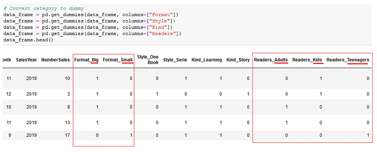<em>Dummies method:</em></strong> This consists in creating a separate column for each single categorical value of a categorical column. As the value of each column is binary (0/1), you can only have one “1” in the newly-generated columns.</p> <p>How to do this in Python:</p> <pre><code># Convert category to dummydata_frame = pd.get_dummies(data_frame, columns=["Format"])data_frame = pd.get_dummies(data_frame, columns=["Style"])data_frame = pd.get_dummies(data_frame, columns=["Kind"])data_frame = pd.get_dummies(data_frame, columns=["Readers"])data_frame.head()</code></pre> <p>You will notice below that “Format” generated 2 columns (“Format_Big” and “Format_Small”), because the “Format” column had 2 single values (“Big” and “Small”). However, “Readers” generated 3 different columns, because it had 3 different values (“Adults”, “Teenagers” and “Kids”).</p> <div> <table cellspacing="0" cellpadding="0"> <tbody> <tr> <th>Id</th> <th>Title</th> <th>Style_Series</th> <th>Style_OneBook</th> <th>Kind_Learning</th> <th>Kind_Story</th> <th>Readers_Adults</th> <th>Readers_Teenagers</th> <th>Readers_Kids</th> <th>Format_Big</th> <th>Format_Small</th> <th>Price</th> <th>Pages</th> <th>SalesMonth</th> <th>SalesYear</th> <th>NumberSales</th> </tr> <tr> <td>1</td> <td>Kids learning book</td> <td>1</td> <td>0</td> <td>1</td> <td>0</td> <td>0</td> <td>0</td> <td>1</td> <td>1</td> <td>0</td> <td>16</td> <td>100</td> <td>11</td> <td>2019</td> <td>10</td> </tr> <tr> <td>2</td> <td>Guts</td> <td>0</td> <td>1</td> <td>0</td> <td>1</td> <td>0</td> <td>0</td> <td>1</td> <td>1</td> <td>0</td> <td>13</td> <td>100</td> <td>12</td> <td>2019</td> <td>3</td> </tr> <tr> <td>3</td> <td>Writing book</td> <td>1</td> <td>0</td> <td>1</td> <td>0</td> <td>1</td> <td>0</td> <td>0</td> <td>1</td> <td>0</td> <td>10</td> <td>120</td> <td>10</td> <td>2019</td> <td>8</td> </tr> <tr> <td>3</td> <td>Writing book</td> <td>1</td> <td>0</td> <td>1</td> <td>0</td> <td>1</td> <td>0</td> <td>0</td> <td>1</td> <td>0</td> <td>10</td> <td>120</td> <td>11</td> <td>2019</td> <td>8</td> </tr> <tr> <td>4</td> <td>Dictation</td> <td>1</td> <td>0</td> <td>1</td> <td>0</td> <td>0</td> <td>1</td> <td>0</td> <td>0</td> <td>1</td> <td>13</td> <td>85</td> <td>9</td> <td>2019</td> <td>22</td> </tr> <tr> <td>4</td> <td>Dictation</td> <td>1</td> <td>0</td> <td>1</td> <td>0</td> <td>0</td> <td>1</td> <td>0</td> <td>0</td> <td>1</td> <td>13</td> <td>85</td> <td>10</td> <td>2019</td> <td>22</td> </tr> </tbody> </table> </div> <p><picture><source srcset="https://mirror.spiria.com/site/assets/files/5792/output_2.400x0.webp" type="image/webp" media="(max-width: 599px)" /><source srcset="https://mirror.spiria.com/site/assets/files/5792/output_2.760x0.webp" type="image/webp" media="(max-width: 999px)" /><source srcset="https://mirror.spiria.com/site/assets/files/5792/output_2.1039x0.webp" type="image/webp" media="(min-width: 1000px)" /><img src="https://mirror.spiria.com/site/assets/files/5792/output_2.png" alt="decorative" /></picture></p> <p>*The “Id” and “Title” columns will not be used during our ML process.</p> <p>The benefit of the dummies method is that all values have the same weight. However, as it adds as many new columns as the number of single categories in each existing column, be cautious of using this method if you already have many columns to consider in the ML process.</p> <p>On the other hand, if you decide to replace your categorical values by numerical ones, it may give more weight to certain categories whose number is higher. For “Readers”, for example, category 3 will impact the result 3 times, as opposed to category 1. You can imagine what can happen when you have many different values in a categorical column.</p> <h3><em>Data Scaling</em></h3> <p>This process will yield numerical data on one common scale, if it is not already the case. It is required when there is a large variation between features ranges. Data Scaling does not apply to <em>label</em> and <em>categorical</em> columns.</p> <p>You have to scale again to have the same weight to all <em>features</em>.</p> <p>In our example, we need to scale the “Price” and “Pages” columns:</p> <ol> <li>Price [10, 16]</li> <li>Pages [85, 120]</li> </ol> <p>These two columns must be scaled, otherwise the “Pages” column will have more weight in the result than the “Price” column.</p> <p>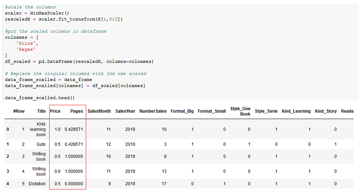While there are many methods of scaling, for the purposes of our example, we used the <code>MinMaxScaler</code> from 0 to 1.</p> <pre><code>#scale the columnsscaler = MinMaxScaler()rescaledX = scaler.fit_transform(X[:,0:2])#put the scaled columns in dataframecolnames = [ 'Price', 'Pages']df_scaled = pd.DataFrame(rescaledX, columns=colnames)# Replace the original columns with the new scaleddata_frame_scalled = data_framedata_frame_scalled[colnames] = df_scaled[colnames]data_frame_scalled.head()</code></pre> <p>The result is the following:</p> <div> <table cellspacing="0" cellpadding="0"> <tbody> <tr> <th>Id</th> <th>Title</th> <th>Style_1</th> <th>Style_2</th> <th>Kind_1</th> <th>Kind_2</th> <th>Readers_1</th> <th>Readers_2</th> <th>Readers_3</th> <th>Format_1</th> <th>Format_2</th> <th>Price</th> <th>Pages</th> <th>NumberSales</th> </tr> <tr> <td>1</td> <td>Kids learning book</td> <td>1</td> <td>0</td> <td>1</td> <td>0</td> <td>0</td> <td>0</td> <td>1</td> <td>1</td> <td>0</td> <td>1</td> <td>0.42857143</td> <td>10</td> </tr> <tr> <td>2</td> <td>Guts</td> <td>0</td> <td>1</td> <td>0</td> <td>1</td> <td>0</td> <td>0</td> <td>1</td> <td>1</td> <td>0</td> <td>0.5</td> <td>0.42857143</td> <td>3</td> </tr> <tr> <td>3</td> <td>Writing book</td> <td>1</td> <td>0</td> <td>1</td> <td>0</td> <td>1</td> <td>0</td> <td>0</td> <td>1</td> <td>0</td> <td>0</td> <td>1</td> <td>8</td> </tr> <tr> <td>4</td> <td>Dictation</td> <td>1</td> <td>0</td> <td>1</td> <td>0</td> <td>0</td> <td>1</td> <td>0</td> <td>0</td> <td>1</td> <td>0.5</td> <td>0</td> <td>22</td> </tr> </tbody> </table> </div> <p><picture><source srcset="https://mirror.spiria.com/site/assets/files/5792/output_3.400x0.webp" type="image/webp" media="(max-width: 599px)" /><source srcset="https://mirror.spiria.com/site/assets/files/5792/output_3.760x0.webp" type="image/webp" media="(max-width: 999px)" /><source srcset="https://mirror.spiria.com/site/assets/files/5792/output_3.1039x0.webp" type="image/webp" media="(min-width: 1000px)" /><img src="https://mirror.spiria.com/site/assets/files/5792/output_3.png" alt="decorative" /></picture></p> <p>As stated, there are many other scaling methods; how and when to use each one will be the subject of a future article.</p>